
Facts and data are the hallmark of good problem solving – but all too often we don’t have enough data or the right kind of data to make good decisions. In Lean Six Sigma we frequently call upon statistical methods, where we know that having an adequate sample size is important.
Simplifying Statistical Jargon
Statistics come with their own rules, vocabulary and seemingly an entire new alphabet. We’ll break down and put into plain terms just what goes into getting enough data when we decide to sample. Ready? Here we go!
What Is Confidence?
In general, we know the more data we have, the more we can depend on the conclusions we draw from that data. Statistically we call this “confidence,” which is expressed as a percentage, such as 95% (a very common confidence). When we draw conclusions from data and have 95% confidence, we can say we are 95% sure that the effect we are observing is real, and not the result of random chance alone. If you deal with very small sample sizes, one sample can give you a very different result than the next and that doesn’t inspire confidence!
One sample can give you a very different result than the next and that doesn’t inspire confidence!
When this happens we’re inclined to take even more samples, and still not be sure what to believe. Having high confidence ensures that each sample is similar enough that we can depend on our observations. This leads to the common question, “How big should my sample be?” The answer is far from simple so let’s see what goes into it…
Too Much Data, or Not Enough?
First of all, let’s consider why we collect data at all – to get information about some situation in order to make improvement choices. The amount of data we need is governed by how much information the data contains. As an example, if you told someone you felt sick, that’s a form of data. Feeling well vs. feeling sick is information that helps them decide what to do for you. But if you told that same person that you had a temperature of 104 degrees Fahrenheit, they might throw you in the car and rush you to the hospital immediately. The temperature data contained a lot more information than just the fact that you felt sick! Temperature has greater information content.
To better understand this concept of the “information content” of data, we’ll consider five different data types.
Qualitative Data: Binary
The simplest discrete data type is binary, where each data point can have only one of two values, such as:
- Good/Bad
- Yes/No
- Pass/Fail
The simplest discrete data type is binary, where each data point can have only one of two values
Binary data has very low “information content” (you don’t know how “bad” or how “good”) – and, as a result, we need more of it to make a decision with much certainty. Consider a coin toss, which can have the value of “heads” or “tails”. If you wanted to find out whether you’re tossing a “fair” coin and not a trick coin you could just toss it a few times. A fair coin would be heads 50% of the time and tails 50% of the time.
Since there are two possible values, you need to toss the coin at least twice. Even if the coin is a fair coin, sometimes you’ll get heads then tails and sometimes you’ll get heads then heads, or tails and tails. On the basis of two flips you can’t be sure if the coin is fair or not. Without going into a lot of mind-numbing statistics (you’re welcome), let me just say that it takes a much larger sample size to have any degree of certainty.
Qualitative Data: Categorical
Categorical data is similar to binary, but can take on more than two values – in fact sometimes many values. It has a little more information content per sample than binary data, but still requires a pretty large sample before you can make decisions with much certainty.
Variable Data: Ordinal
Ordinal data can take on multiple values, but also has order, which provides an additional measure of information. You’ve seen this in in customer surveys. The values are sometimes numerical (as in “Rate this on a Scale from 1 to 5”), or they could be words (“Unacceptable” to “Great”), but there is always a clear sequence of some sort.
Variable Data: Count
Count data typically takes on the form of integers, such as “the number of people on a particular bus” or “the number of crackers in a package.” If the range is small, there is limited information content, but if the range is very large (such as 1-5,000), there is much more information content.
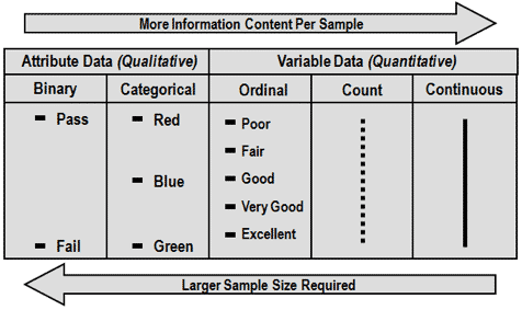
Variable Data: Continuous
Continuous data is typically measured with some kind of gauge (odometer, speedometer, scale, clock, etc.), and is often expressed as a decimal (e.g. 3.25 oz of liquid, 98.6 degrees, etc.). The precision, or number of decimal places depends on the measurement device.
As the arrows show, the greater the information content the fewer the samples needed, and that guides our decision making. We call data on the far left of the diagram Discrete, and on the far right Continuous, with those in between being treated more or less like one of these two major categories.
If our data is Continuous, we might need a sample of a few dozen, whereas for Discrete data we may need hundreds of data points.
So just how much data do you really need? There are two simple answers, but they are somewhat crude and unsatisfying:
- About 30
- The more the better – how much can you get?
The first answer is reasonably correct for Continuous data you can gather easily – it has some statistical justification and often works well. The second answer is a bit trickier, and often comes into play when data is very limited.
So just how much data do you really need? There are two simple answers, but they are somewhat crude and unsatisfying
Examples of Tricky Data Collection
One company manufactured large machined castings. They produced one casting type once every four days, totaling about six a month. It would take five months to gather 30 samples! This is where we simply “take what we can get” and try to make the best of it. Statistical analysis may have to take a back seat to a combination of process knowledge and direct observation.
Another company was looking to improve its invoicing process. All business transactions were logged in a massive database that recorded hundreds of thousands of transactions over many years. In this case there was more than enough data available – the challenge was how to choose the specific samples.
Most of us will find ourselves somewhere between these two extremes, but we still need to know how many samples to collect, and we’d prefer it wasn’t a painful process. Fortunately there are simple formulas for determining sample size.
Fortunately there are simple formulas for determining sample size.
Sample Size Calculation
As we dive into the calculation – we need to meet our new alphabet. The formula here calculates the sample size needed (n) based on the historical standard deviation (s) and the amount of change we would like to be able to detect or precision (Δ), at a confidence of 95%. The measurement units of s and Δ must be the same. Still with me? The good news is that there are lots of sample size calculators out there – but let’s walk through an example.
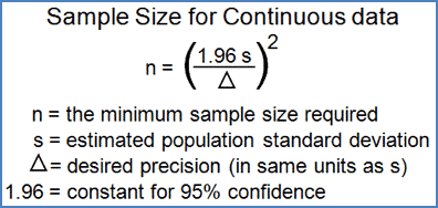
Suppose we are trying to improve the process of month-end-closing of our company financials, and the current process has historically taken 10 hours, with a standard deviation of 2 hours. In terms of sampling the month-end-closings, we would like to detect anything that makes a difference of 6 minutes (a tenth of an hour). We would calculate the sample size (n) by having standard deviation, or s = 2.0 and desired precision, or Δ = 0.1. Once you do the math, the required sample size would be 1537, and since this process only occurs once a month, it would take over 128 years to collect the 1537 samples! Obviously this won’t work, so let’s take a closer look.
Suppose information from other companies indicates that we should be able to cut the process time in half – from 10 hours down to 5 hours. In that case, trying to detect a difference (Δ) of 6 minutes is unrealistic. If we change the Δ to an hour, then the required sample size drops to 16 – a much more achievable number! It will still take more than a year to collect the samples, but if we do some digging through our history, we may be able to find some of what we seek in existing files of past month-end-closing times. That would help limit the number of additional samples needed. But, let’s get back to confidence – what is so special about 95%?
Don’t Be Over Confident!
Years ago the American Management Association (AMA) conducted a study on the accuracy of management decisions. Surprisingly, they found that on average, management only made the right business decisions a little over half the time! That doesn’t mean we have a lot of incompetent managers (though certainly there are some of those), but it does mean that they’re often forced to guess about the future, and they often get it wrong.
Surprisingly, they found that on average, management only made the right business decisions a little over half the time!
So how confident do we need to be? If 95% confidence is overkill, what is the right level? First, consider the consequences of being wrong. Will it damage a customer relationship? Will it shut down the operation? If it could hurt someone, then we need high confidence. If being wrong simply means that we try again – no real damage – then we don’t need as much confidence. The standard 95% confidence gives us 19 to 1 odds of being right – a really good bet! However, a more modest 75% confidence stills gives us 3 to 1 odds of being right – and that’s not a bad bet either.
It’s About Power!
However, there is a key issue missing from the formula which you should always keep in mind when you are looking for clues: power. Whenever we gather information and draw conclusions there are two kinds of mistakes we could make:
- Find something that isn’t real (false positive)
- Miss something that is there (false negative)
Statisticians call the false positive a “Type I Error” and the false negative a “Type II Error.” Both are important. Suppose you visit your doctor for a routine physical exam. They run some tests and share the results. The test results are simply a set of samples that describes our current state of health (blood pressure, cholesterol, blood sugar, etc.).
If there is something wrong and the doctor misses it, it is a “false negative,” and it might mean they missed something critical. Many cancers are difficult to detect in their early stages, when they can more easily be treated – that’s a critical miss!
On the other hand, if the test results indicate a problem which is not real, that’s a “false positive” which could send you into a frightening series of unnecessary tests (doctors seem to love to run more tests!) so that’s a critical Type I Error.
Confidence protects us against “finding” something that isn’t real.
Both types of errors are important, but they’re not necessarily equal. Confidence protects us against “finding” something that isn’t real. If we have 95% confidence, we have only a 5% risk of a false positive.
Power is the probability of detecting something of interest, if it is there. Power protects us against missing something of interest. If we have a 95% power, we have only a 5% risk of a false negative.
As Good As a Coin Toss?
Now here is the “dirty little secret” – the formulas are based on only 50% power! That means that if what you are looking for is really there, you only have a 1 in 2 chance of even finding it. You might as well be flipping a coin!
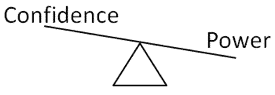
There is a balance between confidence and power. For the same sample size (n) and precision (Δ), the greater the confidence, the less the power, so if we want more power we may have to sacrifice some confidence (assuming we have chosen precision wisely).
Your situation guides you. When we start collecting data, we’re looking for clues. This is when power is most important, and confidence may be almost irrelevant. If we are searching for a cure for cancer we want to find all the clues we can, even if some are false, so we want our power to be high, and our confidence is less important.
Once we find clues, we must carefully investigate the impact of those clues in order to make sure they are real. Before implementing a solution we want to be reasonably sure it will work and that is where confidence becomes much more important than power.
If you really need to keep your sample size low, I suggest reducing your confidence and increasing your power.
If you really need to keep your sample size low, I suggest reducing your confidence and increasing your power. How much? I’ll probably draw some criticism for this, but I’d be comfortable with a confidence of 50% and a power of 80%. If such a low confidence bothers you, try setting both the confidence and power at 75%. There is no simple formula for this, but you can calculate power and sample size using statistical software, such as Minitab, of at the following website:
- For continuous data: http://www.stat.ubc.ca/~rollin/stats/ssize/n1.html
- For binary data: http://stat.ubc.ca/~rollin/stats/ssize/b2.html
Confidence is still important, so don’t ignore it when you are validating root causes or confirming solutions!
Take Charge of Confidence and Make It Work for You!
Summarizing, if you need to minimize your sample size:
- Use continuous data instead of discrete data (where you can)
- Choose a sensible degree of change to detect (Δ) – avoid needless precision!
- Reduce the confidence level to start (but increase it later)
One last thing: if you are fortunate to have lots of data readily available, you can ignore all of this because you have enough for high confidence and high power!
I’ve got the power! (and I’m sure of it).